QuickStart Guide
Installation
To use pyani you will need to install it on a local machine (your laptop, desktop, server or cluster). Installation is easiest using one of the two more popular Python package managers:
1. conda
pyani is available through the bioconda channel of Anaconda:
conda install -c bioconda pyani
2. PyPI
pyani is available via the PyPI package manager for Python:
pip install pyani
Tip
pyani can also be installed directly from source, or run as a Docker image. More detailed, and alternative, installation instructions can be found on the Installation Guide page.
pyani Walkthrough
The general procedure for any pyani analysis is:
- Collect genomes for analysis (and index them)43
- Create a database to hold genome data and analysis results
- Perform ANI/TETRA/etc. analysis
- Report and visualise analysis results
- Generate species hypotheses (classify the input genomes) using the analysis results
To see options available for the pyani program, use the -h
(help) option:
pyani -h
An example ANIm (ANI with MUMmer) analysis using pyani is provided as a walkthrough below. The sequence of commands used is:
pyani download --email my.email@my.domain -t 203804 C_blochmannia
pyani createdb
pyani anim C_blochmannia C_blochmannia_ANIm \
    --name "C. blochmannia run 1" \
    --labels C_blochmannia/labels.txt --classes C_blochmannia/classes.txt
pyani report --runs C_blochmannia_ANIm/ --formats html,excel,stdout
pyani report --run_results 1 --formats html,excel,stdout C_blochmannia_ANIm/
pyani report --run_matrices 1 --formats html,excel,stdout C_blochmannia_ANIm/
pyani plot --formats png,pdf --method seaborn C_blochmannia_ANIm 1
Tip
If you have the pyani source code, you can run the walkthrough commands by executing make walkthrough at the command-line, in the repository root. You can clean up the walkthrough output with make clean_walkthrough.
1. Collect genomes
It is possible to use genomes you have already placed into a local directory with pyani, but for this walkthrough a new set of genomes will be obtained from GenBank, using the pyani download command.
Tip
To read more about using local files with pyani, please see the Indexing Genomes documentation. To read more about downloading genomes from NCBI, please see the Downloading Genomes from NCBI documentation.
Attention
To use their online resources programmatically, NCBI require that you provide your email address for contact purposes if jobs go wrong, and for their own usage statistics. This should be specified with the --email <EMAIL ADDRESS> argument of pyani download.
Using the pyani download subcommand, we download all available genomes for Candidatus Blochmannia from NCBI. The taxon ID for this grouping is 203804, and this ID is passed as the -t argument. The final (compulsory) argument is the path to the directory into which the genome data will be downloaded.
pyani download --email my.email@my.domain -t 203804 C_blochmannia
This creates a new directory (C_blochmannia) with the following contents:
$ tree C_blochmannia
C_blochmannia
├── GCF_000011745.1_ASM1174v1_genomic.fna
├── GCF_000011745.1_ASM1174v1_genomic.fna.gz
├── GCF_000011745.1_ASM1174v1_genomic.fna.md5
[...]
├── GCF_000973545.1_ASM97354v1_hashes.txt
├── classes.txt
└── labels.txt
Each downloaded genome is represented by four files: the genome sequence (FASTA: *.fna, compressed: *.fna.gz), an NCBI hashes file (*_hashes.txt) and an MD5 hash of the genome sequence file (*.md5).
Two additional files are created, summarising all genomes in the subdirectory:
classes.txt: defines a class to which each input genome belongs. This is used for determining membership of groups for each genome, and annotating graphical output.labels.txt: provides text which will be used to label each input genome in the graphical output frompyani
2. Create database
pyani uses a local SQLite3 database to store genome data and analysis results. Existing databases can be re-used. For this walkthrough we create a new, empty database by executing the command:
pyani createdb
Tip
This creates the new database in a default location (.pyani/pyanidb), but the name and location of this database can be controlled with the pyani createdb command (see the Creating a Local pyani Database documentation). The path to the database can be specified in each of the subsequent commands, to enable maintenance and sharing of multiple analysis runs.
3. Conduct ANIm analysis
We run ANIm on the downloaded genomes by specifying first the directory containing the genome data (here, C_blochmannia) then the path to a directory which will contain the analysis results (C_blochmannia_ANIm for this walkthrough).
We also provide a name for the analysis (--name, for later human-readable reference), with optional files defining labels for each genome to be used when plotting output (--labels) and a set of classes to which each genome belongs (--classes) for downstream analysis:
pyani anim C_blochmannia C_blochmannia_ANIm \
    --name "C. blochmannia run 1" \
    --labels C_blochmannia/labels.txt --classes C_blochmannia/classes.txt
This command runs ANIm analysis on the genomes in the specified C_blochmannia directory. As we did not specifiy a database, the analysis results will be stored in the default database we created earlier (.pyani/pyanidb), where they will be identified by the name C. blochmannia run 1. The comparison result files will be written to the C_blochmannia_ANIm directory.
4. Reporting Analyses and Analysis Results
We can list all the runs contained in the (default) database, using the command:
pyani report --runs C_blochmannia_ANIm/ --formats html,excel,stdout
This will report the relevant information to new files in the C_blochmannia_ANIm directory.
$ tree -L 1 C_blochmannia_ANIm/
C_blochmannia_ANIm/
├── nucmer_output
├── runs.html
├── runs.tab
└── runs.xlsx
Tip
By default the pyani report command will create a tab-separated text file with the .tab suffix, but by using the --formats option, we have also created an HTML file, and an Excel file with the same data. The stdout option also prints the output table to the terminal window.
By inspecting the runs.tab file (or any of the other runs.* files) we see that our walkthrough analysis has run ID 1. So we can use this ID to get tables of specific information for that run, such as:
the genomes that were analysed in all runs
pyani report --runs_genomes --formats html,excel,stdout C_blochmannia_ANIm/
the complete set of pairwise comparison results for a single run (listed by comparison)
pyani report --run_results 1 --formats html,excel,stdout C_blochmannia_ANIm/
comparison results as matrices (percentage identity and coverage, number of aligned bases and “similarity errors”, and a Hadamard matrix of identity multiplied by coverage).
pyani report --run_matrices 1 --formats html,excel,stdout C_blochmannia_ANIm/
Attention
The --run_results and --run_matrices options take a single run ID or a comma-separated list of IDs (such as 1,3,4,5,9) as an argument, and will produce output for each specified run ID.
Graphical output
Graphical output is obtained by executing the pyani plot subcommand, specifying the output directory and run ID. Optionally, output file formats and the graphics drawing method can be specified.
pyani plot --formats png,pdf --method seaborn C_blochmannia_ANIm 1
Supported output methods are:
seabornmpl(matplotlib)plotly
and each generates five plots corresponding to the matrices that pyani report produces:
- percentage identity of aligned regions
- percentage coverage of each genome by aligned regions
- number of aligned bases on each genome
- number of “similarity errors” on each genome
- a Hadamard matrix of percentage identity multiplied by percentage coverage for each comparison
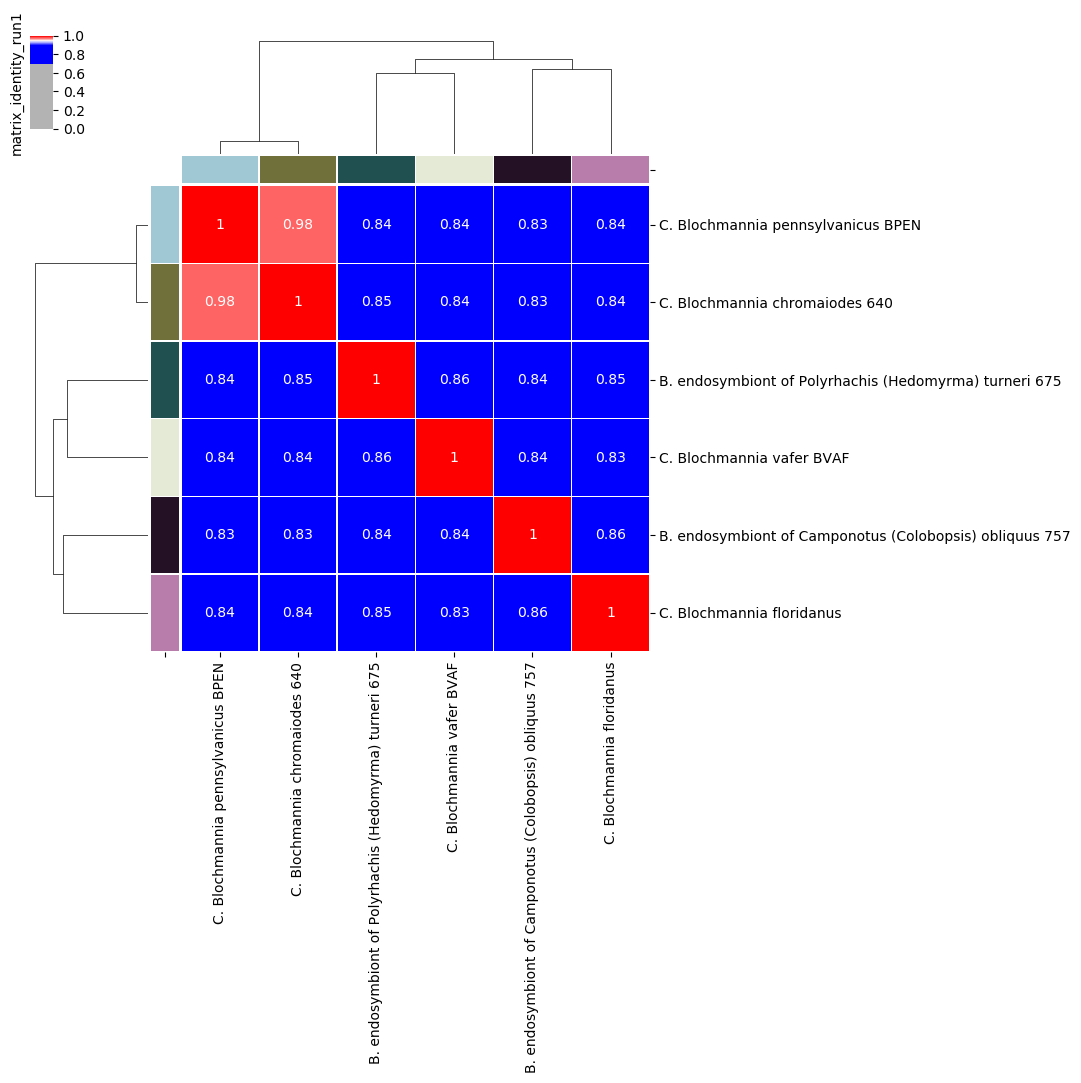
Percentage identity matrix for Candidatus Blochmannia ANIm analysis
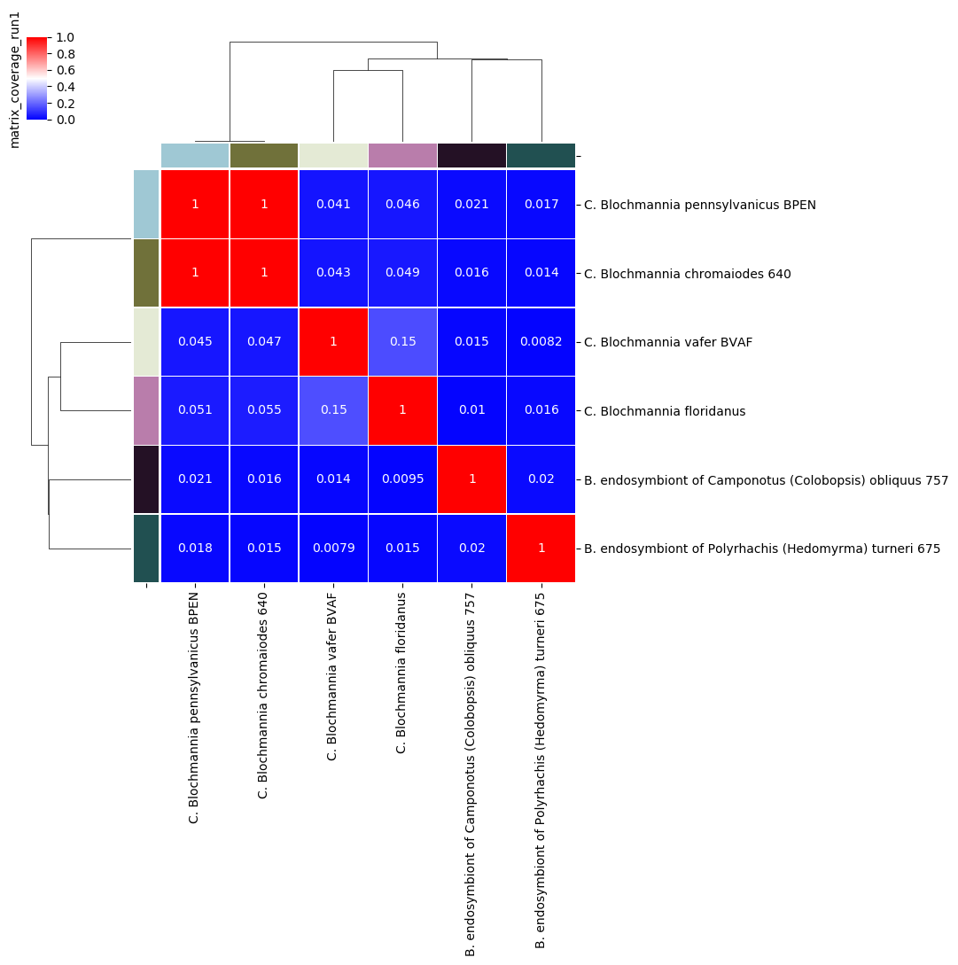
Percentage coverage matrix for Candidatus Blochmannia ANIm analysis
Several graphics output formats are available, including .png, .pdf and .svg.